Basic Properties of Electromagnetic Waves
Why I am writing about Maxwell's Equations while there are so many formal manuals: It is a way to repeat what I learned from the subject, and to make sure that I understood each expression used.
I started getting to Maxwell's Equations deep meanings when I came to the Telecommunication school and took additional EM course to discover the richness of these equations that govern the telecommunication world. I wanted to
put out a summary for anyone who wants to read and enjoy these equations that Maxwell had put together. It is not a complete guide, but will keep adding additional definitions.
Maxwell's Equations
Maxwell's equations provide a mathematical model for electric, optical, and radio technologies such as power generation, electrical motor, and wireless communication. Maxwell's equations encompass the major laws of electricity and magnetism. Maxwell's equations did not appeared alone suddenly, rather they appeared in accordance with the time spirit of a request under the leap of electric technology and the development of science and technology by the industrial revolution. Maxwell derived the Maxwell's equations as a mathematical equation from the result of Faraday's experimental and theoretical study. He has not only developed the science and technology of the era of that time, but also opened a new world.The existence of propagating electromagnetic waves can be predicted as a direct consequence of Maxwell's equations, which is the very basics of radio communication and of satellites communications [iida2013satellite]. Maxwell's equation of the electromagnetic wave is a collection of four equations, e.g. Gauss's law of electrostatic, Gauss's law of magnetism, Faraday's law of electromotive force, and Ampere's Circuital law. Maxwell converted the integral form of these equations into the differential form of the equations. The differential form of these equations is known as Maxwell's equations. These equations specify the relationships between the variations of the vector electric field \(\textbf{E}\) and the vector magnetic field \(\textbf{B}\) in time and space within a medium [saunders2007antennas]. Note that this section does not aim to provide rigorous or complete derivation of Maxwell's equations. For a fuller treatment, see books such as [kraus1977electromagnetics]
Maxwell's four equations can be summarized as [zhang1990electromagnetic,schelkunoff1955conversion, becherrawy2013electromagnetism, kopriva2000discontinuous, kletzing2013electric, hajnal1990observations,jian2000electromagnetic]\begin{align} & &\vec{\nabla} \cdot \vec{\textbf{E}} = \frac{\rho}{\epsilon_0} &\mbox{(Gauss' law of electrostatic)} [eq:GLE]\\ & &\vec{\nabla} \cdot \vec{\textbf{B}} = 0 & \mbox{(Gauss' law of magnetism)} [eq:GLM]\\ & &\vec{\nabla} \times \vec{\textbf{E}} = -\frac{\partial \vec{\textbf{B}}}{\partial t} &\mbox{(Faraday's law of electromotive force)} [eq:FLEF]\\ %& &\vec{\nabla} \times \vec{\textbf{B}} = \vec{\textbf{J}} + \frac{\partial \vec{\textbf{D}}}{\partial t} &\mbox{(Maxwell-Ampere law)} \\ & &\vec{\nabla} \times \vec{\textbf{B}} = \mu\vec{\textbf{J}} + \mu\epsilon\frac{\partial \vec{\textbf{E}}}{\partial t} &\mbox{(Maxwell-Ampere law)} [eq:MAL] \end{align} where \(\vec{\textbf{E}}\) is the electric field, \(\vec{\textbf{B}}\) the magnetic field, \(\rho\) the charge density, \(\vec{\textbf{J}}\) is the current density, \(\epsilon_0\) the permittivity in free space, \(\mu\) the permeability of the medium.
The above equations can be interpreted as follows:
Equation [eq:GLE]: Divergence of electric field is equal to the number of charges density per volume. If there is a volume, with more positive charges than negative, the divergence of the electric field will be positive. If there are more negative than positive charges, then the divergence is negative. If the volume has equal amount of positive and negative charges, then the divergence is zero.
Equation [eq:GLM]: The divergence of magnetic field is always equal to zero. Although you can have more positive or negative electric charges, for magnet, you can't have more north than south, or more south than north. Following the magnetic lines, they can't never converge or diverge from a point. They curl around in circles. The assumption is that there are no magnetic monopoles.
Equation [eq:FLEF]: The changing in a magnetic field will create an electric field that curls around the changing of magnetic field. To the negative sign meaning, the curling electric field is in a conductor. It will create its own circling current, which according to Ampere's law, will make its own curling magnetic field. The negative sign means that the magnetic field from the current will push against the changing external magnetic field. If the negative sign was not there, you could not only build a perpetual motion machine, but build a perpetual motion machine that constantly accelerates.
Equation [eq:MAL]: The curl of a magnetic field is either due to the current the magnetic field is circling, or from a changing electric field that is inducing a perpendicular magnetic field around it. A circulating magnetic field is produced by an electric current, and by an electric field that changes with time.
Lorentz Force Law: \begin{equation} \vec{\textbf{F}}_{EM} = q(\vec{\textbf{E}} + \vec{\textbf{v}} \times \vec{\textbf{B}}) \end{equation} where \(\vec{\textbf{F}}_{EM}\) stands for electromagnetic force, \(q\) the test charge, \(\vec{\textbf{v}}\) the velocity of the test charge moving through the magnetic field, and \(\vec{\textbf{B}}\) the magnetic field.
For free space:Current density \((\vec{\textbf{J}}=0)\)
Volume charge distribution \((\rho)=0\)
Permittivity \(\epsilon=\epsilon_0\)
Permeability \(\mu=\mu_0\)
Now, Maxwell's equation for free space: \begin{align} & &\vec{\nabla} \cdot \vec{\textbf{E}} = 0 \label{eq:FSGLE} \\ & &\vec{\nabla} \cdot \vec{\textbf{B}} = 0 \label{eq:FSGLM} \\ & &\vec{\nabla} \times \vec{\textbf{E}} = -\frac{\partial \vec{\textbf{B}}}{\partial t} \label{eq:FSFLEF} \\ & &\vec{\nabla} \times \vec{\textbf{B}} = \mu_{0}\epsilon_{0}\frac{\partial \vec{\textbf{E}}}{\partial t} \label{eq:FSMAL} \\ \end{align} On solving the Maxwell's equations for free space, the electromagnetic wave equations for free space are derived (Eq. [eq:FSGLE] - [eq:FSMAL]) . Recall that the electromagnetic wave equation has both an electric field vector and a magnetic field vector. Therefore, Maxwell's equations for free space give two-equation for electromagnetic wave: the electric field vector \((\vec{\textbf{E}})\) and the magnetic field vector \((\vec{\textbf{B}})\).
Electromagnetic wave equation in free space in term of \(\vec{\textbf{E}}\)
From equation [eq:FLEF], take the curl on both sides [danielmmittleman]:\(\vec{\nabla} \times [(\vec{\nabla} \times \vec{\textbf{E}})] = \vec{\nabla} \times [-\frac{\partial \vec{\textbf{B}}}{\partial t}]\)
Change the order of differentiation on the right hand side:
\begin{equation} \vec{\nabla} \times [(\vec{\nabla} \times \vec{\textbf{E}})] = -\frac{\partial}{\partial t} [\vec{\nabla} \times \vec{\textbf{B}}] \end{equation} But equation [eq:MAL], \(\vec{\nabla} \times \vec{\textbf{B}} = \mu\epsilon\frac{\partial \vec{\textbf{E}}}{\partial t}\)
Substituting for \(\vec{\nabla} \times \vec{\textbf{B}}\), we have:
\(\vec{\nabla} \times [(\vec{\nabla} \times \vec{\textbf{E}})] = -\frac{\partial}{\partial t} [\vec{\nabla} \times \vec{\textbf{B}}] \longrightarrow \vec{\nabla} \times [(\vec{\nabla} \times \vec{\textbf{E}})] = -\frac{\partial}{\partial t} [\mu\epsilon\frac{\partial \vec{\textbf{E}}}{\partial t}]\)
Or:
\(\vec{\nabla} \times [(\vec{\nabla} \times \vec{\textbf{E}})] = - \mu\epsilon \frac{\partial^{2} \vec{\textbf{E}}}{\partial t^{2}}\)
It can be shown that:
\(\vec{\nabla} \times [(\vec{\nabla} \times \vec{\textbf{E}})]\)
is the same as:
\(\vec{\nabla} (\vec{\nabla}\cdot \vec{\textbf{E}}) - \vec{\nabla}^{2} \vec{\textbf{E}}\)
For any function at all,
\begin{equation} \vec{\nabla}(\vec{\nabla}\cdot \vec{\textbf{F}}) - \nabla^{2} \vec{\textbf{F}} = \vec{\nabla} \times [(\vec{\nabla} \times \vec{\textbf{F}})] \end{equation} Assume now zero charge density, \(\rho=0$, then: $\vec{\nabla} \cdot \vec{\textbf{E}} = 0\)
Therefore,
\begin{equation} \nabla^{2} \vec{\textbf{E}} = \mu\epsilon \frac{\partial^{2} \vec{\textbf{E}}}{\partial t^{2}} \end{equation} is the electromagnetic wave equation for free space in terms of electric field vector \((\vec{\textbf{E}})\)
Electromagnetic wave equation in free space in term of \(\vec{\textbf{B}}\)
Using the previous subsection approach, a wave equation for the magnetic field is derived: \begin{equation} \nabla^{2} \vec{\textbf{B}} = \mu\epsilon \frac{\partial^{2} \vec{\textbf{B}}}{\partial t^{2}} \end{equation} 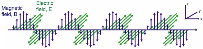 |
\(\vec{\textbf{E}}\) and \(\vec{\textbf{B}}\) satisfy the same equation. However, it does not mean they are equal. \(\vec{\textbf{E}}\) and \(\vec{\textbf{B}}\) are always perpendicular to each other (Figure EM-waves). In Figure [fig:EM-waves] illustrations, the vectors of the two fields, electric and magnetic, are only shown at a few selected locations, equally spaced along a line. But the fields are defined at every point (x,y,z). Additional definitions on vectors, curl, and divergence can be found in the next section.
Proof \(\vec{\textbf{E}}\) and \(\vec{\textbf{B}}\) are orthogonal to the wave vector:
... coming soon ...
Complement: Vector, Divergence, Gradient, Curl
Divergence, gradient and curl are vectors derivative that appear in Maxwell's equation. Their definitions and meaning are given in this section.
The "Del" operator:
\begin{equation*} \vec{\nabla} \equiv \begin{pmatrix} \frac{\partial}{\partial x}, \frac{\partial}{\partial y}, \frac{\partial}{\partial z} \end{pmatrix} =\frac{\partial}{\partial x}\hat{x} + \frac{\partial}{\partial y}\hat{y} + \frac{\partial}{\partial z}\hat{z} \end{equation*}The "Gradient" of a scalar function \(f\):
\begin{equation*} \vec{\nabla}f \equiv \begin{pmatrix}\frac{\partial f}{\partial x}, \frac{\partial f}{\partial y}, \frac{\partial f}{\partial z}\end{pmatrix} \end{equation*} The gradient points in the direction of steepest ascent.The "Divergence" of a vector function \(\vec{G}\):
\begin{equation*} \vec{\nabla}\cdot\vec{G} \equiv \frac{\partial G_{x}}{\partial x}+ \frac{\partial G_{y}}{\partial y}+ \frac{\partial G_{z}}{\partial z} \end{equation*}The "Laplacian" of a scalar function:
\begin{equation*} \nabla^{2}f \equiv \vec{\nabla}\cdot\vec{\nabla}f = \vec{\nabla}\cdot \begin{pmatrix}\frac{\partial f}{\partial x},\quad \frac{\partial f}{\partial y},\quad \frac{\partial f}{\partial z}\end{pmatrix} = \frac{\partial^{2}f}{\partial x^{2}} + \frac{\partial^{2}f}{\partial y^{2}} + \frac{\partial^{2}f}{\partial z^{2}} \end{equation*}The Laplacian of a vector function is the same, but for each component:
\begin{equation*} \nabla^{2}\vec{G} = \begin{pmatrix}\frac{\partial^{2}G_{x}}{\partial x^{2}} + \frac{\partial^{2}G_{x}}{\partial y^{2}} + \frac{\partial^{2}G_{x}}{\partial z^{2}},\quad \frac{\partial^{2}G_{y}}{\partial x^{2}} + \frac{\partial^{2}G_{y}}{\partial y^{2}} + \frac{\partial^{2}G_{y}}{\partial z^{2}},\quad \frac{\partial^{2}G_{z}}{\partial x^{2}} + \frac{\partial^{2}G_{z}}{\partial y^{2}} + \frac{\partial^{2}G_{z}}{\partial z^{2}} \end{pmatrix} \end{equation*} The Laplacian is related to the curvature of a function.The "Curl" of a vector function \(\vec{G}\):
\begin{equation*} \vec{\nabla}\times\vec{G} \equiv \begin{pmatrix}\frac{\partial G_{z}}{\partial y} - \frac{\partial G_{y}}{\partial z},\quad \frac{\partial G_{x}}{\partial z} - \frac{\partial G_{z}}{\partial x},\quad \frac{\partial G_{y}}{\partial x} - \frac{\partial G_{x}}{\partial y}\end{pmatrix} \end{equation*} The curl can be computed from a matrix determinant: \begin{equation*} \vec{\nabla}\times\vec{G} = \det \begin{bmatrix} \hat{\textbf{x}} & \hat{\textbf{y}} & \hat{\textbf{z}}\\ \frac{\partial}{\partial x} & \frac{\partial}{\partial y} & \frac{\partial}{\partial z}\\ G_{x} & G_{y} & G_{z} \end{bmatrix} \end{equation*} The curl measures the microscopic circulation of the vector field.Practical Realization of Radio Communication
In the 19th century, numerous inventors and scientists, including Michael Faraday, James Clerk Maxwell, Heinrich Rudolf Hertz, Nikola Testla, David Edward Hughes, Thomas Edison, and Guglielmo Marconi, began to experiment with wireless communications. These innovators discovered and created many theories about the concepts of electrical magnetic radio frequency (RF) [coleman2012cwna].
German physicist Heinrich Rudolf Hertz (1857-1894) clarified Maxwell's electromagnetism theory more and developed it. He made the equipment which generated the electromagnetic wave and the detected existence of emission of an electromagnetic wave in 1888 and demonstrated it through experiments of distance of 12 meters [iida2013satellite]. Hertz's experiments confirmed that an electromagnetic wave is a transverse wave, propagates at limited speed (velocity of light), and has properties such as propagating through the various materials, a reflection, refraction, and deflection the same as light [iida2013satellite].
Guglielmo Marconi (1874-1937) succeeded in the first radio communication in the world in 1895. The transmitter and receiver (coherer wave detector) themselves are not originally created by Marconi, but an antenna in top and the ground earth bottom are originally developed by Marconi. He succeeded a long distance communication of 1.5 kilometers [iida2013satellite].
Wireless networking technology was first used by the US military during World War II to transmit data over an RF medium using classified encryption technology to send battle plans across enemy lines. In the 1970, the University of Hawaii developed the first wireless network called ALOHAnet, to wirelessly communicate data between the Hawaiian Islands. In the 1990, commercial networking vendors began to produce low-speed wireless data networking products, most of which operated in the 900 MHz frequency band. The Institute of Electrical and Electronics Engineers (IEEE) began to discuss standardizing WLAN technologies in 1991. In 1997, the IEEE ratified the original 802.11 standard that is the foundation of the wireless local area network (WLAN) technologies [coleman2012cwna].