Antenna Array Beamforming Demystification
Array-element Signal Formulation
Antenna array signal processing is an actively developing research area in communication technologies and
connected to the progress in optimization theory, and remains the key technological development that
attracts more than one.
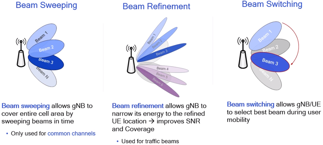
Beamforming is a signal processing operation that uses antenna arrays to create a spatial filter. Beamforming
consists to filter out signals from all directions except the desired direction(s). Beamforming can be used
to increase SINR (signal-to-interference-plus-noise ratio) of desired signals, null out interferers, shape
beam patterns, or even transmit/receive multiple data streams at the same time and frequency (5G & 6G).
 |
|---|
Antenna arrays have a huge role in radar, where the goal is to detect and track targets.
This module introduces the theory in narrowband array signal processing beamforming and direction of arrival estimation algorithms and the basic principle of array signal processing techniques to further understand its implementation process and applications.
Assumptions of the signal mathematical model used in beamforming and DOA estimation algorithms:
- Each array element is an ideal omnidirectional point source, and the inter-element spacing is less than or equal to half-a-wavelength
- Signal sources are assumed to be in the far-field so that the signals impinging on the array can be regarded as a plane wave
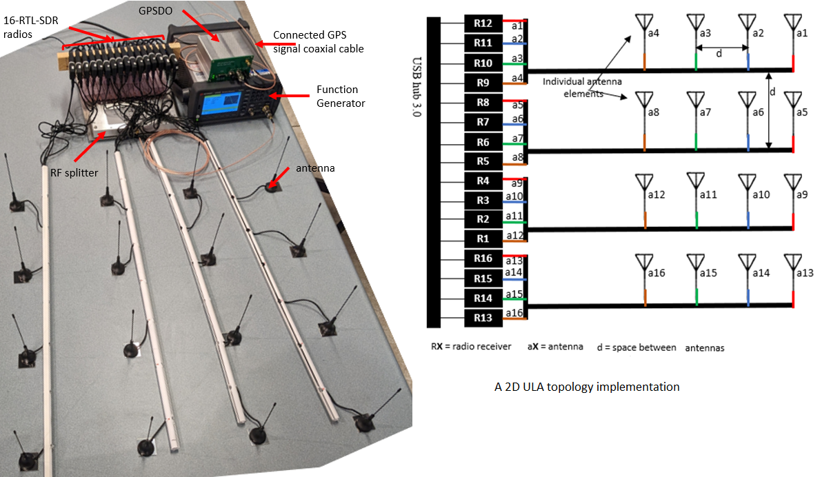
- Let us consider a uniform linear array (ULA) topology. Spacing between array elements are equal, e.g. evenly spaced array
- The noise is zero-mean Gaussian white noise, and uncorrelated with the signal source
- The effect of mutual coupling between array elements is assumed to be negligible, i.e., the different element receives the same signal amplitude.
 |
|---|
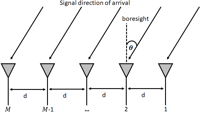
In Fig. 2, a signal is coming in from the right side (pure assumption). It is hitting the right-most element first. Consider the signal received by the first array element as a reference signal, then the analytical expression for the i−th signal received with respect to the reference array element is
\( s_i (t) = m_i (t) e^{j2\pi f_c t}, i = 0, ..., P-1\) (Eq. 1)
where \(m_i (t)\) is the complex envelope of the \( i-th\) modulated signal, and \( f_c\) the carrier frequency.
The signal received by each array element has a certain delay relative to the origin of the coordinates. The delay between when the signal hits that first element and when it reaches the next element can be calculated by forming the trigonometry problem formulated from Fig.2.
 |
|---|
\( cos(90 - \theta) = \frac{adjacent}{hypotenuse} = \frac{adjacent}{d}\)
\( adjacent = d * cos(90 - \theta) = d * sin(\theta)\) Remember: cos(a - b) = cos(a)cos(b) + sin(a)sin(b)
The adjacent is just a distance. Convert the adjacent-distance to a time is necessary by using the speed of light: \( time_{elapsed} = d \sin(\theta) / c \). This equation applies between any adjacent elements of the array.
The propagation delay of the received signal from reference array element to the \( m−th \) array element can be expressed as
\( \tau_m (\theta_i) = \frac{d}{c} (m-1) sin(\theta_i)\) \( m=1, ..., M \) (Eq. 2)
According to (Eq. 1), the signal received at the \(m-th\) array element is the superposition of all signals and can be expressed as:
\(x_m (t) = \sum_{i=0}^{P-1} m_i (t-\tau_m (\theta_i)) e^{j2\pi f_c (t-\tau_m (\theta_i))} + n_m (t) \) (Eq. 3-a)
where \(n_m (t)\) is the Gaussian noise signal received at the \(m-th\) array element having zero mean and variance \(\sigma^2\). Recall that when you have a time shift, it is subtracted from the time argument. (Eq. 3-a) can be rewritten:
\(x_m (t) = \sum_{i=0}^{P-1} m_i (t-\tau_m (\theta_i)) e^{j2\pi f_c t} e^{-j2\pi f_c \tau_m (\theta_i)} + n_m (t) \) (Eq. 3-b)
Because the carrier component in the system does not affect the analysis, and the adaptive algorithm is often carried out in the baseband or complex envelope, the carrier part in the above equation can be ignored. The remaining can be expressed as:
\(x_m (t) = \sum_{i=0}^{P-1} m_i (t-\tau_m (\theta_i)) e^{-j2\pi f_c \tau_m (\theta_i)} + n_m (t) \) (Eq. 3-c)
Since we consider a narrowband signal source located in the far-field, the bandwidth \(B\) of the signal satisfy the condition \(B<< f_c \), and \(m_i (t)\) changes relatively slowy because the signal delay is \(\tau_m (\theta_i) << \frac{1}{B}\). Therefore, the complex envelope of the signal can be approximated as \(m_i (t-\tau_m (\theta_i))\approx m_i (t)\)
\(x_m (t) = \sum_{i=0}^{P-1} m_i (t) e^{-j2\pi f_c \tau_m (\theta_i)} + n_m (t) \) (Eq. 3-d)
A little detail:
\(k=\frac{2\pi f_c}{c}\) \(f_c=\frac{kc}{2\pi}\) where \(k\) is the free space wave number
Recall \( \tau_m (\theta_i) = \frac{d}{c} (m-1) sin(\theta_i)\)
Replacing the above details into (Eq. 3.d) gives:
\(x_m (t) = \sum_{i=0}^{P-1} m_i (t) e^{-j(m-1)kd sin \theta_i} + n_m (t) \) (Eq. 3-e)
At time \(t\), the overall received signal can be expressed as:
\begin{equation} x(t) = \begin{bmatrix} x_1 (t)\\x_2 (t)\\.\\x_M (t) \end{bmatrix} = Am (t) + n(t) (Eq. 4-a) \end{equation}
\begin{equation} x(t) = \begin{bmatrix} 1 & 1 & ... & 1 \\ e^{-jkd sin\theta_0} & e^{-jkd sin\theta_1} & ... & e^{-jkd sin\theta_{P-1}} \\ . & . & . & .\\ . & . & . & .\\ . & . & . & .\\ e^{-j(M-1)kd sin\theta_0} & e^{-j(M-1)kd sin\theta_1} & ... & e^{-j(M-1)kd sin\theta_{P-1}} \end{bmatrix} \begin{bmatrix} m_1 (t) \\ m_2 (t) \\ . \\ . \\ . \\ m_p (t) \end{bmatrix} + \begin{bmatrix} n_1 (t) \\ n_2 (t) \\ . \\ . \\ . \\ n_M (t) \end{bmatrix} (Eq. 4-b) \end{equation}
Hence, from Eq. 4-b, we can define:
For instance: \(a(\theta_0) = [1 e^{-jkd sin \theta_0)} ... e^{-j(M-1)kd sin \theta_0)}]^T\)
The array response vector, a 2D array, is a function of the angle of arrival, individual element response, the array geometry, and the signal frequency (Fig. 4). The first element of the steering vector is always 1, e.g. \(e^0 = 1\), and the rest are phase shifts relative to the first element. The steering vector is used in DOA.
 |
|---|
Beamforming
Why beamforming? Beamforming is used to
RF Beamforming is to estimate the desired signal properties by adjusting the complex weights at each sensor applied to the received signal which result in enhancement of desired signal and place nulls in the direction of interference. Description will be made based on digital beamforming system.
 |
|---|
Array processing objectives
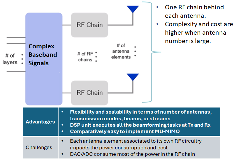
In digital beamforming, each array element has a dedicated ADC. The received signals from each element are multiplied by the conjugates of the weights \(w_m\) and then summed. The weighted signals are added together to form the output signal. Using these weights, a weighted response can be defined. The weights are allowed to change, depending on the received data, to achieve a purpose. In addition, the signal at each element is corrupted by thermal noise modeled as additive white Gaussian noise. The output received signal is therefore given by \begin{equation} y(t) = w^H x(t) = \sum_{m=1}^{M} w_{m}^{*} x_m (t) (Eq. 5) \end{equation} where \(w^H = [w_0^*, w_1^*, ..., w_{M-1}^*]\)
Optimal Beamforming
In beamforming, the weight vector is computed by solving the optimization of the cost function. The different cost functions corresponds to different criteria. Some of the most frequently used performance criteria’s include minimum mean squared error (MMSE), maximum likelihood (ML). As the weights are iteratively adjusted, the cost function becomes smaller and smaller. When the cost function is minimized, the performance criterion is met and the algorithm is said to have converged.Minimum Mean Squared Error
Mean squared error refers to the mean squared difference between the beamformer output and the desired signal.
The MMSE algorithm minimizes the error with respect to a reference signal x(t). If the signal prior knowledge
is known, the receiver can generate a local reference signal which has a strong correlation with the desired
signal. The main idea of MMSE is to adjust the weight vector in real time, so that the mean squared error
between the array output signal and the reference signal can be minimized.
From Eq. 4-a, the received signals is expressed as
\begin{equation}
y= Am + n = Hx + n (Eq. 6)
\end{equation}
where \(m \in \mathbb{C}^{N_t \times 1} \) represent the input signal,
\(A \in \mathbb{C}^{N_r \times N_t} \) the channel response,
\(n \in \mathbb{C}^{N_r \times 1}\) the observation noise. Note that \(N_t\) and \(N_r\) are respectively the number
of transmitting and receiving antennas.
Let's define the following:
We seek to estimate \(x\):
General Orthogonality Principle:
Goal: Find an estimator \(W\) such that the pdf for the error \(e\) is orthogonal to the data \(y\): \(E[ey^H]=0\).
If the error \(e\) is statistically independent of the observed data \(y\), then there is nothing further one can do with the observed data to determine the error, and therefore to reduce the error. In this case, the estimator W(ꞏ) is optimal (i.e., it can’t be improved upon).
The above applies not only to temporal data, but also to spatial data, volume data, and any other multidimensional data (even "big" data!).
A MMSE tries to minimize the mean square error (MSE) of the residual error \(e=\hat{x}-x\).
Now, let's connect the above formulas:
\(E[ey^H]=0\)
\(E[(\hat{x}-x)y^H]=0\)
\(E[(W_{MMSE}y-x)y^H]=0\)
\(E[W_{MMSE}yy^H-xy^H]=0\) Let's say \(W_{MMSE}=W\), and Using Eq. 6, we have
\(E[W(Hx + n)(Hx + n)^H-x(Hx + n)^H]=0\)
\(E[W(Hxx^HH^H + Hxn^H + H^Hnx^H + nn^H) -xx^HH^H - xn^H]=0\)
\(WE[Hxx^HH^H] + WE[Hxn^H] + WE[H^Hnx^H] + WE[nn^H] -E[xx^HH^H] - E[xn^H]=0\)
\(WHR_{xx}H^H + WHR_{xn} + WH^HR_{nx} + WR_{nn} -R_{xx}H^H - R_{xn}=0\)
\(WHR_{xx}H^H + 0 + 0 + WR_{nn} - R_{xx}H^H - 0 =0\)
\(W(HR_{xx}H^H + R_{nn}) = R_{xx}H^H \)
\begin{equation} W_{MMSE} = R_{xx}H^H (HR_{xx}H^H + R_{nn})^{-1} (Eq. 7) \end{equation}
MUltiple SIgnal Classification - MUSIC
Definitions are coming soon!  |
|---|
MORE TO COME SOON ...next will be MUSIC ...